ACTIVE Network API Developer Blog

Building a Predictive Model

Multinomial Naive Bayes (NB) Classifier

The Support Vector Machine (SVM)

Support vector machines² are popular and very powerful methods for classification. The general idea is to draw some sort of separating line between populations of data which maximizes their separation, given a set of constraints, by maximizing the "margin" — the distance of that separator from the nearest training data point. The data can be mapped to higher dimensions using the "kernel trick" to achieve better separation:


Of course, there are many ways to define and draw a line, but the fastest is a straight line and the linear SVMs are quite fast. By altering variables in the algorithm, you can adjust how this line is drawn, favoring things like good overall separation (large margin) over classification mistakes in the training data (error rate). Adjusting this trade-off is called "regularization", and amounts to adjusting the size and complexity of how the margin is represented. You may still want the best separating line even if some data points are on the wrong side or in the space between. However, as you test lines, you may want to penalize these data points, and you may want to do that differently depending on what the error was. This is done with so called "loss" functions. Varying regularization and loss functions affects results, but also processing time (both in training and in testing, and not necessarily the same way).

When you add functions to regularize or compute loss, you are also adding points of variability where you can decide to do more. The Passive-Agressive⁴ algorithm is one such modifier which acts passively for data points with no loss according to some loss function, and aggressively with data points causing loss, to varying extents, to modify the loss function.


This guarantees that there is some non-zero margin at each update and means it can also be performed online. This was an addition Google made to weed out search result spam (2004-2005) and reduced it by 50%.

Scoring

Ensembles

from sklearn.naive_bayes import MultinomialNB
from sklearn.linear_model import SGDClassifier, PassiveAggressiveClassifier
models = []
models.append(MultinomialNB(alpha=.01)) 
models.append(SGDClassifier(alpha=.0001, loss='modified_huber',n_iter=50,n_jobs=-1,random_state=42,penalty='l2'))
models.append(PassiveAggressiveClassifier(C=1,n_iter=50,n_jobs=-1,random_state=42)) 

from sklearn.externals import joblib
from sklearn import metrics
results = {}
for model in models:
    model_name = type(model).__name__
    model.fit(X_train, Y_train)
    joblib.dump(model, "models/topics."+model_name+".pkl")
    pred = model.predict(X_test)
    class_f1 = metrics.f1_score(Y_test, pred, average=None)
    model_f1 = metrics.f1_score(Y_test, pred)
    model_acc = metrics.accuracy_score(Y_test, pred)
    probs = None
    norm = False
    try:
        probs = model.predict_proba(X_test)
    except:
        pass
    if probs is None:
        try:
            probs = model.decision_function(X_test)
            norm = True
        except:
            print "Unable to extract probabilities"
            pass
        pass
    results[model_name] = { "pred": pred, 
                            "probs": probs, 
                            "norm": norm, 
                            "class_f1": class_f1, 
                            "f1": model_f1, 
                            "accuracy": model_acc }
results    

{'MultinomialNB': {'accuracy': 0.90317052270779774,
  'class_f1': array([ 0.91176471,  0.78378378,  0.92307692,  1.        ,  0.73226545,
        0.98550725,  1.        ,  0.92727273,  0.83783784,  0.66666667,
        0.92307692,  0.96551724,  0.96969697,  0.7826087 ,  0.81818182,
        0.94117647,  0.80952381,  0.95652174,  0.90740741,  0.72727273,
        0.8       ,  0.90909091,  0.88888889,  0.85714286,  0.82848837,
        0.84615385,  0.91542289,  1.        ,  0.93167702,  0.9375    ,
        1.        ,  0.95238095,  0.90909091,  0.85714286,  1.        ,
        0.9       ,  0.90909091,  0.77777778,  0.9       ,  0.89189189,
        0.92134831,  0.9       ,  0.99386503,  0.96296296,  1.        ,
        0.81481481,  1.        ,  1.        ,  1.        ,  0.9726776 ,
        0.88888889,  0.81481481,  1.        ,  0.93506494,  0.66666667,
        1.        ,  0.9       ,  0.66666667,  0.77727952,  0.92307692,
        0.88461538,  0.86956522,  0.88479263,  0.93023256,  0.95302013,
        0.88888889,  0.91428571,  1.        ,  0.78571429,  0.81818182,
        0.95238095,  0.95238095,  1.        ,  0.8       ,  0.92134831,
        0.75      ,  0.9       ,  0.95686275,  0.84210526,  0.92307692,
        0.92982456,  0.90909091,  0.975     ,  0.98630137,  0.83333333,
        1.        ,  1.        ,  0.99043977,  0.76923077,  0.76923077,
        0.72      ,  0.66666667,  1.        ,  0.92561983,  0.76923077,
        0.86842105,  0.6728972 ,  1.        ,  1.        ,  0.9819376 ,
        0.92030848]),
  'f1': 0.90425650714576233,
  'norm': False,
  'pred': array([ 80.,  34.,  40., ...,  80.,  80.,  99.]),
  'probs': array([[  2.40973619e-073,   4.61021751e-072,   1.49431625e-083, ...,
          7.06802900e-070,   7.87538237e-085,   3.95436935e-092],
       [  3.84477547e-009,   2.73354066e-009,   5.04147141e-009, ...,
          5.64165086e-009,   4.27726628e-010,   6.96643800e-010],
       [  1.35237976e-033,   1.55981122e-026,   5.27750168e-031, ...,
          1.38907003e-031,   1.91871068e-040,   7.90134376e-023],
       ..., 
       [  7.00464283e-021,   1.42085525e-019,   1.08346607e-027, ...,
          8.18649153e-026,   7.52087143e-027,   4.42046005e-023],
       [  1.04982806e-049,   1.33612621e-047,   5.33165094e-045, ...,
          8.20836489e-049,   2.76637762e-060,   1.15624776e-058],
       [  4.77707280e-230,   6.78060805e-227,   2.04462450e-214, ...,
          4.03932473e-212,   1.00000000e+000,   9.62285611e-258]])},
 'PassiveAggressiveClassifier': {'accuracy': 0.91533847472150809,
  'class_f1': array([ 0.86956522,  0.85714286,  1.        ,  1.        ,  0.6450116 ,
        0.98550725,  1.        ,  0.92592593,  0.90909091,  0.90909091,
        1.        ,  0.96551724,  0.96969697,  0.81818182,  0.9       ,
        0.875     ,  0.97142857,  1.        ,  0.92982456,  0.88888889,
        0.85714286,  0.88888889,  1.        ,  1.        ,  0.86111111,
        0.88      ,  0.97354497,  1.        ,  0.92215569,  0.96774194,
        1.        ,  1.        ,  0.76923077,  0.86075949,  0.98876404,
        0.97560976,  1.        ,  0.94117647,  0.94736842,  0.92715232,
        0.92045455,  0.78947368,  0.98159509,  0.94871795,  1.        ,
        0.775     ,  1.        ,  1.        ,  1.        ,  0.97777778,
        0.88      ,  0.88      ,  1.        ,  0.86567164,  1.        ,
        1.        ,  0.84210526,  0.66666667,  0.85557084,  0.93333333,
        0.89361702,  0.91304348,  0.91402715,  0.95348837,  0.94520548,
        0.91304348,  0.8       ,  1.        ,  0.89655172,  0.76923077,
        0.93023256,  0.95081967,  1.        ,  1.        ,  0.93478261,
        0.8       ,  0.95238095,  0.99230769,  0.92307692,  0.96296296,
        0.92156863,  0.90909091,  0.96202532,  1.        ,  0.86746988,
        0.97560976,  0.97297297,  0.98846154,  0.75555556,  0.83333333,
        0.9       ,  0.8       ,  1.        ,  0.94736842,  0.9375    ,
        0.9382716 ,  0.7804878 ,  1.        ,  1.        ,  0.98846787,
        0.95187166]),
  'f1': 0.91627947823867106,
  'norm': True,
  'pred': array([ 80.,  34.,  24., ...,   4.,  80.,  99.]),
  'probs': array([[-6.50553156, -7.33053267, -5.86251708, ..., -6.3615013 ,
        -4.61827337, -4.99723938],
       [-1.42865833, -1.30183262, -1.276344  , ..., -1.28003285,
        -1.32275774, -1.53379058],
       [-1.86725075, -2.50969362, -1.77919327, ..., -1.79010457,
        -1.74044571, -1.64161697],
       ..., 
       [-2.10958176, -1.57150069, -2.75524001, ..., -3.05243249,
        -2.32612049, -2.33553294],
       [-2.85613606, -5.13216583, -3.12312947, ..., -3.39208034,
        -3.37134486, -2.82044267],
       [-4.74802868, -8.87368108, -5.07165789, ..., -4.46875551,
         4.16080753, -6.87427149]])},
 'SGDClassifier': {'accuracy': 0.91088260497000861,
  'class_f1': array([ 0.92307692,  0.79411765,  1.        ,  1.        ,  0.67613636,
        0.97142857,  1.        ,  0.93883792,  0.94117647,  0.71428571,
        0.97142857,  0.96551724,  0.96969697,  0.80952381,  0.94736842,
        0.82352941,  0.94444444,  0.97777778,  0.91076923,  0.88888889,
        0.94117647,  0.93333333,  1.        ,  0.85714286,  0.84709066,
        0.84615385,  0.94972067,  1.        ,  0.93251534,  0.85714286,
        1.        ,  1.        ,  1.        ,  0.85333333,  1.        ,
        0.95238095,  1.        ,  0.94117647,  0.94736842,  0.91275168,
        0.93491124,  0.81081081,  0.98765432,  0.94871795,  1.        ,
        0.79487179,  0.96774194,  1.        ,  1.        ,  0.97206704,
        0.83333333,  0.84615385,  0.95652174,  0.88888889,  1.        ,
        1.        ,  0.83333333,  0.66666667,  0.82099596,  0.91479821,
        0.83333333,  0.88372093,  0.92727273,  0.94382022,  0.97183099,
        0.93023256,  0.875     ,  0.95652174,  0.93333333,  0.86956522,
        0.95238095,  0.95081967,  0.8       ,  1.        ,  0.87058824,
        0.8       ,  0.95238095,  0.9765625 ,  0.86486486,  0.96296296,
        0.91327148,  0.66666667,  0.98734177,  0.95652174,  0.89156627,
        0.97560976,  0.96363636,  0.97475728,  0.80952381,  0.8       ,
        0.95238095,  0.75      ,  1.        ,  0.96491228,  0.9375    ,
        0.95121951,  0.72941176,  1.        ,  1.        ,  0.98839138,
        0.94933333]),
  'f1': 0.91022607629402619,
  'norm': True,
  'pred': array([ 80.,  34.,  40., ...,  80.,  80.,  99.]),
  'probs': array([[ -2.26147719,  -8.27192811,  -4.92650663, ...,  -6.28101298,
         -4.394243  ,  -5.40679641],
       [ -5.28684017,  -6.85913339,  -6.07070456, ...,  -6.38595219,
         -4.88673419,  -8.5894273 ],
       [ -5.44502194,  -7.45632928,  -6.12684297, ...,  -6.38543615,
         -5.01141554,  -8.79847179],
       ..., 
       [ -3.62707077,  -5.61320527,  -5.65215132, ...,  -6.35567368,
         -5.028778  ,  -8.08235843],
       [ -5.02315463,  -7.26758048,  -5.8154445 , ...,  -6.52950791,
         -5.16125362,  -9.12372876],
       [ -6.22352808,  -7.47187108,  -6.1562682 , ...,  -6.45018436,
          6.56404494, -11.14563358]])}}

def normalize_distances(probs):
    # get the probabilities of a positive and negative distance
    pPos = float(len(np.where(np.array(probs) > 0)[0])) / float(len(probs))
    pNeg = float(len(np.where(np.array(probs) < 0)[0])) / float(len(probs))
    if pNeg > 0:
        probs[np.where(probs > 0)] *= pNeg
    if pPos > 0:
        probs[np.where(probs < 0)] *= pPos
    # subtract the mean and divide by standard deviation if non-zero
    probs_std = np.std(probs, ddof=1)
    if probs_std != 0:
        probs = (probs - np.mean(probs)) / probs_std
    # divide by the range if non-zero
    pDiff = np.abs(np.max(probs) - np.min(probs))
    if pDiff != 0:
        probs /= pDiff
    return probs

def compute_confidence(probs, labels, norm=False):
    confidences = None
    class_confidence = []
    if norm:
        confidences = normalize_distances(probs)
    else:
        confidences = probs
    for c in xrange(len(confidences)):
        confidence = round(confidences[c], 2)
        if confidence != 0:
            class_confidence.append({ "label": labels[c], "confidence": confidence })
    return sorted(class_confidence, key=lambda k: k["confidence"], reverse=True)

def predict(txt, model, model_name, vectorizer, labels):
    predObj = {}
    X_data = vectorizer.transform([txt])
    pred = model.predict(X_data)
    label_id = int(pred[0])
    predObj["model"] = model_name
    predObj["label_name"] = labels[label_id]
    predObj["f1_score"] = float(results[model_name]["class_f1"][label_id])
    if results[model_name]["norm"]:
        probs = model.decision_function(X_data)[0]
    else:
        probs = model.predict_proba(X_data)[0]
    predObj["confidence"] = compute_confidence(probs, labels, norm=results[model_name]["norm"])
    return predObj
    
    
        

prediction_results = []
label_scores = None
model_names = []
txt = "This is a tough mud run. Tough, as in, this could be one of the hardest events you, as a runner have ever attempted. This is not a walk in the park. This is not your average neighborhood 5k. This is more fun than a marathon. This is a challenge. The obstacles were designed by military and fitness experts and will test you to the max. Push personal limits while running, crawling, climbing, jumping, dragging, and other surprise tasks that test endurance and strength. The race consists of non-competitive heats as well as a free kid's course for children age 5-13. Each heat will depart in a specific wave so the course doesn't get overcrowded."
for model in models:
    model_name = type(model).__name__
    try:
        prediction_results.append( predict(txt,
                                    model,model_name, vectorizer, unique_topics))
        model_names.append(model_name)
    except Exception, e:
        print "Error predicting" + str(e)
        pass
prediction_results

[{'confidence': [{'confidence': 1.0, 'label': u'Mud running'}],
  'f1_score': 0.6666666666666665,
  'label_name': u'Mud running',
  'model': 'MultinomialNB'},
 {'confidence': [{'confidence': 0.94, 'label': u'Distance running'},
   {'confidence': 0.14, 'label': u'Mud running'},
   {'confidence': 0.01, 'label': u'Bassoon'},
   {'confidence': 0.01, 'label': u'Dance'},
   {'confidence': 0.01, 'label': u'Judo'},
   {'confidence': 0.01, 'label': u'Sexual health'},
   {'confidence': 0.01, 'label': u'Strength training'},
   {'confidence': 0.01, 'label': u'Tuba'},
   {'confidence': -0.01, 'label': u'Acting'},
   {'confidence': -0.01, 'label': u'Aikido'},
   {'confidence': -0.01, 'label': u'Bowling'},
   {'confidence': -0.01, 'label': u'Chess'},
   {'confidence': -0.01, 'label': u'Child care'},
   {'confidence': -0.01, 'label': u'Chinese'},
   {'confidence': -0.01, 'label': u'Cross country skiing'},
   {'confidence': -0.01, 'label': u'Digital photography'},
   {'confidence': -0.01, 'label': u'Diving'},
   {'confidence': -0.01, 'label': u'Drawing and drafting'},
   {'confidence': -0.01, 'label': u'Driving'},
   {'confidence': -0.01, 'label': u'Fencing'},
   {'confidence': -0.01, 'label': u'Flag football'},
   {'confidence': -0.01, 'label': u'Ice hockey'},
   {'confidence': -0.01, 'label': u'Italian'},
   {'confidence': -0.01, 'label': u'Kayaking'},
   {'confidence': -0.01, 'label': u'Knitting'},
   {'confidence': -0.01, 'label': u'Painting'},
   {'confidence': -0.01, 'label': u'Percussion and Drumming'},
   {'confidence': -0.01, 'label': u'Pilates'},
   {'confidence': -0.01, 'label': u'Reading and writing'},
   {'confidence': -0.01, 'label': u'Sculpture'},
   {'confidence': -0.01, 'label': u'Self-defence'},
   {'confidence': -0.01, 'label': u'Skateboarding'},
   {'confidence': -0.01, 'label': u'Table tennis'},
   {'confidence': -0.01, 'label': u'Taxes'},
   {'confidence': -0.01, 'label': u'Tending animals'},
   {'confidence': -0.01, 'label': u'Theater'},
   {'confidence': -0.01, 'label': u'Violin'},
   {'confidence': -0.01, 'label': u'Wrestling'},
   {'confidence': -0.02, 'label': u'Aerobics'},
   {'confidence': -0.02, 'label': u'Ballroom dance'},
   {'confidence': -0.02, 'label': u'CPR'},
   {'confidence': -0.02, 'label': u'Cello'},
   {'confidence': -0.02, 'label': u'Cross country running'},
   {'confidence': -0.02, 'label': u'First aid and CPR'},
   {'confidence': -0.02, 'label': u'Improv'},
   {'confidence': -0.02, 'label': u'Mountain biking'},
   {'confidence': -0.02, 'label': u'Photography'},
   {'confidence': -0.02, 'label': u'Pottery and ceramics'},
   {'confidence': -0.02, 'label': u'Snowboarding'},
   {'confidence': -0.02, 'label': u'Spanish'},
   {'confidence': -0.02, 'label': u'Tae Kwon Do'},
   {'confidence': -0.02, 'label': u'Tap dance'},
   {'confidence': -0.02, 'label': u'Tennis'},
   {'confidence': -0.02, 'label': u'Tumbling'},
   {'confidence': -0.03, 'label': u'Aquatic sports'},
   {'confidence': -0.03, 'label': u'Creative writing'},
   {'confidence': -0.03, 'label': u'Flute'},
   {'confidence': -0.03, 'label': u'Ice skating'},
   {'confidence': -0.03, 'label': u'Jewelry making'},
   {'confidence': -0.03, 'label': u'Karate'},
   {'confidence': -0.03, 'label': u'Skiing'},
   {'confidence': -0.03, 'label': u'Voice and singing'},
   {'confidence': -0.03, 'label': u'Zumba'},
   {'confidence': -0.04, 'label': u'Ballet'},
   {'confidence': -0.04, 'label': u'Hip Hop dance'},
   {'confidence': -0.04, 'label': u'Jazz dance'},
   {'confidence': -0.04, 'label': u'Lifeguarding'},
   {'confidence': -0.05, 'label': u'Guitar'},
   {'confidence': -0.06, 'label': u'Piano'}],
  'f1_score': 0.9497206703910615,
  'label_name': u'Distance running',
  'model': 'SGDClassifier'},
 {'confidence': [{'confidence': 0.6, 'label': u'Mud running'},
   {'confidence': 0.43, 'label': u'Distance running'},
   {'confidence': 0.25, 'label': u'Strength training'},
   {'confidence': 0.24, 'label': u'Chess'},
   {'confidence': 0.21, 'label': u'Cross country running'},
   {'confidence': 0.2, 'label': u'Lifeguarding'},
   {'confidence': 0.17, 'label': u'Sailing'},
   {'confidence': 0.17, 'label': u'Trail running'},
   {'confidence': 0.16, 'label': u'Mountain biking'},
   {'confidence': 0.16, 'label': u'Skateboarding'},
   {'confidence': 0.15, 'label': u'Zumba'},
   {'confidence': 0.14, 'label': u'Acting'},
   {'confidence': 0.14, 'label': u'Yoga'},
   {'confidence': 0.12, 'label': u'Badminton'},
   {'confidence': 0.11, 'label': u'Snowboarding'},
   {'confidence': 0.11, 'label': u'Surfing'},
   {'confidence': 0.1, 'label': u'Cake decorating'},
   {'confidence': 0.1, 'label': u'Karate'},
   {'confidence': 0.09, 'label': u'Archery'},
   {'confidence': 0.09, 'label': u'Drawing and drafting'},
   {'confidence': 0.09, 'label': u'Judo'},
   {'confidence': 0.09, 'label': u'Wood work'},
   {'confidence': 0.08, 'label': u'Kayaking'},
   {'confidence': 0.08, 'label': u'Piano'},
   {'confidence': 0.07, 'label': u'Aikido'},
   {'confidence': 0.07, 'label': u'Snowshoeing'},
   {'confidence': 0.07, 'label': u'Tai chi'},
   {'confidence': 0.06, 'label': u'Diving'},
   {'confidence': 0.06, 'label': u'Ice skating'},
   {'confidence': 0.06, 'label': u'Quilting'},
   {'confidence': 0.06, 'label': u'Tae Kwon Do'},
   {'confidence': 0.05, 'label': u'Chinese'},
   {'confidence': 0.04, 'label': u'Flute'},
   {'confidence': 0.04, 'label': u'French'},
   {'confidence': 0.04, 'label': u'Kickboxing'},
   {'confidence': 0.04, 'label': u'Percussion and Drumming'},
   {'confidence': 0.04, 'label': u'Pilates'},
   {'confidence': 0.04, 'label': u'Wrestling'},
   {'confidence': 0.03, 'label': u'Bridge'},
   {'confidence': 0.03, 'label': u'Driving'},
   {'confidence': 0.03, 'label': u'Fencing'},
   {'confidence': 0.03, 'label': u'Guitar'},
   {'confidence': 0.03, 'label': u'Tap dance'},
   {'confidence': 0.02, 'label': u'Cello'},
   {'confidence': 0.02, 'label': u'Digital photography'},
   {'confidence': 0.02, 'label': u'Saxophone'},
   {'confidence': 0.02, 'label': u'Tumbling'},
   {'confidence': 0.01, 'label': u'American football'},
   {'confidence': 0.01, 'label': u'Bowling'},
   {'confidence': 0.01, 'label': u'French horn'},
   {'confidence': 0.01, 'label': u'Improv'},
   {'confidence': 0.01, 'label': u'Jazz dance'},
   {'confidence': 0.01, 'label': u'Sexual health'},
   {'confidence': 0.01, 'label': u'Taxes'},
   {'confidence': -0.01, 'label': u'First aid and CPR'},
   {'confidence': -0.01, 'label': u'Tennis'},
   {'confidence': -0.01, 'label': u'Trombone'},
   {'confidence': -0.01, 'label': u'Trumpet'},
   {'confidence': -0.02, 'label': u'Ballroom dance'},
   {'confidence': -0.02, 'label': u'Cross country skiing'},
   {'confidence': -0.02, 'label': u'Field hockey'},
   {'confidence': -0.02, 'label': u'Magic'},
   {'confidence': -0.02, 'label': u'Pottery and ceramics'},
   {'confidence': -0.02, 'label': u'Viola'},
   {'confidence': -0.02, 'label': u'Violin'},
   {'confidence': -0.03, 'label': u'Self-defence'},
   {'confidence': -0.04, 'label': u'Photography'},
   {'confidence': -0.05, 'label': u'Ballet'},
   {'confidence': -0.05, 'label': u'Italian'},
   {'confidence': -0.06, 'label': u'Boxing'},
   {'confidence': -0.08, 'label': u'Gardening'},
   {'confidence': -0.08, 'label': u'Hip Hop dance'},
   {'confidence': -0.09, 'label': u'Spanish'},
   {'confidence': -0.1, 'label': u'Table tennis'},
   {'confidence': -0.1, 'label': u'Theater'},
   {'confidence': -0.11, 'label': u'Jewelry making'},
   {'confidence': -0.14, 'label': u'Reading and writing'},
   {'confidence': -0.15, 'label': u'Creative writing'},
   {'confidence': -0.15, 'label': u'Ice hockey'},
   {'confidence': -0.15, 'label': u'Voice and singing'},
   {'confidence': -0.16, 'label': u'Figure skating'},
   {'confidence': -0.17, 'label': u'CPR'},
   {'confidence': -0.18, 'label': u'Painting'},
   {'confidence': -0.19, 'label': u'Tending animals'},
   {'confidence': -0.25, 'label': u'Flag football'},
   {'confidence': -0.27, 'label': u'Dance'},
   {'confidence': -0.27, 'label': u'Skiing'},
   {'confidence': -0.28, 'label': u'Aquatic sports'},
   {'confidence': -0.32, 'label': u'Child care'},
   {'confidence': -0.36, 'label': u'Aerobics'},
   {'confidence': -0.36, 'label': u'Swimming'},
   {'confidence': -0.37, 'label': u'Music'},
   {'confidence': -0.4, 'label': u'Sculpture'}],
  'f1_score': 0.6666666666666666,
  'label_name': u'Mud running',
  'model': 'PassiveAggressiveClassifier'}]

from operator import itemgetter
conf_labels = {}
scored_labels = {}
for prediction_result in prediction_results:
    if "label_name" in prediction_result:
        l_name = prediction_result["label_name"]
        f1_score = prediction_result["f1_score"]
        conf = [ float(c["confidence"]) for c in prediction_result["confidence"] if c["label"] == prediction_result["label_name"] ]
        if len(conf):
            conf = conf[0]
        else:
            conf = 0
        # update with confidence weighted by f1
        #variations are to *= f1_score, or update confidence with just the confidence
        if l_name in scored_labels.keys():
            conf_labels[l_name] += f1_score * conf
            scored_labels[l_name] += f1_score
        else:
            conf_labels[l_name] = f1_score * conf
            scored_labels[l_name] = f1_score
labels_sorted = sorted(scored_labels.iteritems(),key=itemgetter(1),reverse=True)
labels_pred = []
# compute ensemble averages
num_models = len(models)
for i in xrange(len(labels_sorted)):
    label = labels_sorted[i][0]
    label_avg_f1score = float("%0.3f" % (float(labels_sorted[i][1]) / num_models))
    label_avg_conf = float("%0.3f" % (float(conf_labels[label]) / num_models))
    label_score = float("%0.3f" % (label_avg_f1score * label_avg_conf))
    labels_pred.append({ "label": label, "score": label_score })
labels_pred = sorted(labels_pred, key=lambda k: k["score"], reverse=True)
labels_pred   

[{'label': u'Mud running', 'score': 0.158},
 {'label': u'Distance running', 'score': 0.094}]

Asset Processing Overview

Asset Topics

Prediction API

Right tools for the job

• → Can process 200k or more documents rapidly (in seconds) for vectorization (n-gram counts, tf/idf, scaling, SVD/PCA, hashing, etc.)
• → Offers lots of well-maintained and vetted algorithms for classification (SVM and linear SVM, self-organizing maps and other neural network methods, Bayes and other statistical and probabilistic learning techniques, tree-based methods, etc.)
• → Provides measures of performance, parameter sweeping, and lots of stats
• → Enables multiclass (as opposed to binary) and multilabel (“green” and “fast” as opposed to “green” or “fast”) prediction options
• → Amenable to a prediction ensemble setup (combining different algorithms)

• → Sparse matrices support
  • › 150k assets with 20k features = 3x10^9 matrix members
• → Optimized parallel processing (threads and processes)
  • › We need models in minutes and predictions in milliseconds

• → Fast to support inclusion of prediction in the asset processing workflow, or any other place
• → Support for proxy and reverse proxy (like nginx)
• → Security
• → JSON support
• → Pre-forking and event loop support

• → As new data comes in
  • › reach a threshold
  • › rebuild models
  • › self-assess
  • › plug and deploy or rebuild with new parameters
• → As issues arise

• → Unsupervised clustering
• → similarity algorithms for recommendations
• → custom classification and clustering algorithm development

• → Devs without a data science background should be able to:
  • › plug in new DS-derived functions
  • › create new web server routes and API endpoints
  • › adjust API output
  • › add and apply basic stats and counting
  • › code review
• → Data scientist devs should be able to extend it easily

Java

Ruby

R and MATLAB

Combos

Python

{ "event": { "topic": "Hip Hop dance", "text": "Pre-School Tumbling/ Hip Hop    " } }
{ "event": { "topic": "Distance running", "text": "Santito Youth Talent Ministry Mile Run/Walk    " } }
{ "event": { "topic": "Yoga", "text": "Pre/Post-Natal Yoga M Yoga is an ideal form of exercise before, during, and after pregnancy, and is safe and nurturing, Maintain strength and flexibility, combat fatigue, swelling, back ache and nausea, calm nerves and increase relaxation while reducing common discomforts. Moms and babies welcome. Instructor: Dana Chamblin.  " } }
{ "event": { "topic": "Dance", "text": "Cardio Line Dancing at Haines This activity takes line dancing to a whole new level. Get a cardiovascular workout and learn a variety of moves and experience many genres of music.  " } }
{ "event": { "topic": "Distance running", "text": "The 32nd Annual Skunk Cabbage Classic Run Preregistration: $20, must be postmarked by Friday, February 15, 2013; $25.00 from February16, 2013-April 8th, 2013. Race day registration $35 until 9:45 a.m. race day.  " } }
{ "event": { "topic": "Photography", "text": "Photography Class with Ron St. Germain Whether your camera is an old one from the closet or the newest technology, this class will familiarize you with all of its buttons and functions. You will learn the basics in a fun and easily understood way with entertaining slide presentations and plenty of time to ask questions each week from 5-time International Award winning outdoor photographer, Ron St. Germain. For detailed information, check his website at  www.daphotodude.com .  " } }
{ "event": { "topic": "Creative writing", "text": "Memoir Writing (6/27-7/18)    Memoirs are your memories. Learn how to convert your memories into interesting stories to pass down to future generations. Participants will learn how to connect with the great, great, great grandchildren that they will never meet and show them what their lives were like.   " } }
{ "event": { "topic": "Yoga", "text": " Fall Exercise, 01a Mommy   Me (Mon)    " } }

import json, re

def clean(txt):
    #clean your data (strip tags, remove number-only words, etc.)
    return txt

def loadCorpus(data_file):
    labels = []
    texts = []
    #load your data
    events = open(data_file).readlines()
    cnt = 0
    processed = 0
    for d in xrange(len(events)):
        cnt += 1
        event = re.sub(r'(\n|\r)+','',events[d].strip())
        try:
          json_event = json.loads(event, 'utf-8')
          event = json_event["event"]
          labels.append(event["topic"])
          texts.append(clean(event["text"]))
          processed += 1
        except Exception, e:
          pass
    print str(processed) + " events processed out of " + str(cnt) + " (" + str(float(processed)/float(cnt)) + ")!"
    return labels,texts

labels_train,data_train = loadCorpus("topics_events.json")

116717 events processed out of 120475 (0.968806806391)!

import numpy as np

# index the topics, getting unique entries with Python's set object
unique_topics = list(set(labels_train))
unique_topics.sort()
labels_train = np.array(labels_train)
labels = np.empty(shape=labels_train.shape)
for c in xrange(len(unique_topics)):
    # use numpy's where function to find and index topics
    labels[np.where(labels_train == unique_topics[c])] = c

X_train = data_train
# set aside test data using about 5% of the full data set
data_len = len(X_train)
tsn = int(data_len*0.05)
# generate a random set of indexes to pluck out for testing
test_samp = np.random.randint(0,data_len,tsn)
# use Python's list comprehension so pull out test data and labels
X_test = [ X_train[i] for i in test_samp ]
Y_test = [ labels[i] for i in test_samp ]
# remove the test data from the training data
Y_train = list(labels)
for s in sorted(test_samp,reverse=True):
    del X_train[s]
    del Y_train[s]

print str(len(X_train)) + " training docs, " + str(len(X_test)) + " testing docs"
print "Topics:"
[str(ut) for ut in unique_topics]

110882 training docs, 5835 testing docs
Topics:
['Acting',
 'Aerobics',
 'Aikido',
 'American football',
 'Aquatic sports',
 'Archery',
 'Badminton',
 'Ballet',
 'Ballroom dance',
 'Bassoon',
 'Bowling',
 'Boxing',
 'Bridge',
 'CPR',
 'Cake decorating',
 'Card games',
 'Cello',
 'Chess',
 'Child care',
 'Chinese',
 'Clarinet',
 'Creative writing',
 'Cross country running',
 'Cross country skiing',
 'Dance',
 'Digital photography',
 'Distance running',
 'Diving',
 'Drawing and drafting',
 'Driving',
 'Fencing',
 'Field hockey',
 'Figure skating',
 'First aid and CPR',
 'Flag football',
 'Flute',
 'French',
 'French horn',
 'Gardening',
 'Guitar',
 'Hip Hop dance',
 'Ice hockey',
 'Ice skating',
 'Improv',
 'Italian',
 'Jazz dance',
 'Jewelry making',
 'Jiu-jitsu',
 'Judo',
 'Karate',
 'Kayaking',
 'Kickboxing',
 'Knitting',
 'Lifeguarding',
 'Magic',
 'Massage',
 'Mountain biking',
 'Mud running',
 'Music',
 'Painting',
 'Percussion and Drumming',
 'Photography',
 'Piano',
 'Pilates',
 'Pottery and ceramics',
 'Quilting',
 'Reading and writing',
 'Sailing',
 'Saxophone',
 'Sculpture',
 'Self-defence',
 'Sewing',
 'Sexual health',
 'Skateboarding',
 'Skiing',
 'Snowboarding',
 'Snowshoeing',
 'Spanish',
 'Strength training',
 'Surfing',
 'Swimming',
 'Table tennis',
 'Tae Kwon Do',
 'Tai chi',
 'Tap dance',
 'Taxes',
 'Tending animals',
 'Tennis',
 'Theater',
 'Trail running',
 'Trombone',
 'Trumpet',
 'Tuba',
 'Tumbling',
 'Viola',
 'Violin',
 'Voice and singing',
 'Wood work',
 'Wrestling',
 'Yoga',
 'Zumba']

from sklearn.feature_extraction.text import CountVectorizer
vectorizer = CountVectorizer(stop_words='english',charset_error='ignore',ngram_range=(1,3),min_df=2) 
X_train = vectorizer.fit_transform(X_train)
X_train

<110882x479646 sparse matrix of type '<type 'numpy.int64'>'
	with 5200668 stored elements in COOrdinate format>

X_test = vectorizer.transform(X_test)
X_test

<5835x479646 sparse matrix of type '<type 'numpy.int64'>'
	with 247403 stored elements in COOrdinate format>

from sklearn.naive_bayes import MultinomialNB
model = MultinomialNB(alpha=.01)
model.fit(X_train, Y_train)

MultinomialNB(alpha=0.01, class_prior=None, fit_prior=True)

from sklearn.externals import joblib
joblib.dump(model, "models/topics.MultinomialNB.pkl")

['models/topics.MultinomialNB.pkl',
 'models/topics.MultinomialNB.pkl_01.npy',
 'models/topics.MultinomialNB.pkl_02.npy',
 'models/topics.MultinomialNB.pkl_03.npy']

# do the prediction
pred = model.predict(X_test)
print pred

[ 64.   4.  42. ...,  43.  58.  26.]

# get some performance metrics
from sklearn import metrics

# scores per class, output not printed here to save space
#print  metrics.f1_score(Y_test, pred, average=None)
#print  metrics.recall_score(Y_test, pred, average=None) 
#print  metrics.precision_score(Y_test, pred, average=None) 
  

# overall scores
print  metrics.f1_score(Y_test, pred)
print  metrics.accuracy_score(Y_test,pred)

# performance by topic
print  metrics.classification_report(Y_test, pred,target_names=unique_topics)
print "Confusion Matrix:"
print  metrics.confusion_matrix(Y_test, pred)

0.899494891223
0.898886032562
                         precision    recall  f1-score   support

                 Acting       0.97      1.00      0.99        36
               Aerobics       0.77      0.73      0.75        37
                 Aikido       1.00      1.00      1.00         5
      American football       1.00      1.00      1.00        13
         Aquatic sports       0.65      0.76      0.70       186
                Archery       0.97      1.00      0.99        37
              Badminton       1.00      0.93      0.97        15
                 Ballet       0.84      0.97      0.90       301
         Ballroom dance       0.80      0.94      0.86        47
                Bassoon       0.25      1.00      0.40         2
                Bowling       0.94      0.94      0.94        18
                 Boxing       1.00      0.86      0.92         7
                 Bridge       0.90      1.00      0.95         9
                    CPR       0.71      0.79      0.75        19
        Cake decorating       0.89      0.67      0.76        12
             Card games       1.00      1.00      1.00         2
                  Cello       0.72      1.00      0.84        18
                  Chess       0.92      1.00      0.96        12
             Child care       0.96      0.90      0.93       156
                Chinese       0.93      0.87      0.90        15
               Clarinet       0.86      1.00      0.92         6
       Creative writing       0.85      1.00      0.92        28
  Cross country running       0.83      0.83      0.83         6
   Cross country skiing       0.62      1.00      0.77         5
                  Dance       0.90      0.75      0.82       425
    Digital photography       0.76      0.93      0.84        14
       Distance running       0.82      0.99      0.90        97
                 Diving       0.92      1.00      0.96        11
   Drawing and drafting       0.94      0.93      0.94       105
                Driving       1.00      1.00      1.00        15
                Fencing       0.83      1.00      0.91        10
           Field hockey       0.93      0.93      0.93        15
         Figure skating       0.88      0.88      0.88         8
      First aid and CPR       0.85      0.88      0.87        33
          Flag football       1.00      0.92      0.96        38
                  Flute       0.62      1.00      0.76        13
                 French       0.67      1.00      0.80         6
            French horn       0.71      0.83      0.77         6
              Gardening       1.00      0.83      0.91        12
                 Guitar       0.88      0.90      0.89        87
          Hip Hop dance       0.83      0.92      0.87        78
             Ice hockey       1.00      0.82      0.90        11
            Ice skating       0.98      0.98      0.98        88
                 Improv       0.87      0.94      0.91        36
                Italian       1.00      1.00      1.00         7
             Jazz dance       0.71      0.79      0.75        62
         Jewelry making       0.90      1.00      0.95        18
              Jiu-jitsu       0.82      1.00      0.90         9
                   Judo       0.50      0.50      0.50         2
                 Karate       0.98      0.99      0.98        80
               Kayaking       0.91      0.83      0.87        12
             Kickboxing       1.00      1.00      1.00        11
               Knitting       0.86      0.86      0.86         7
           Lifeguarding       0.89      0.93      0.91        43
                  Magic       0.83      1.00      0.91         5
                Massage       1.00      0.89      0.94         9
        Mountain biking       0.91      0.78      0.84        27
            Mud running       1.00      0.82      0.90        11
                  Music       0.91      0.73      0.81       350
               Painting       0.93      0.93      0.93       134
Percussion and Drumming       0.90      0.90      0.90        30
            Photography       0.95      0.83      0.89        24
                  Piano       0.88      0.92      0.90       104
                Pilates       0.85      0.90      0.88        31
   Pottery and ceramics       0.96      0.94      0.95        69
               Quilting       0.94      1.00      0.97        17
    Reading and writing       1.00      0.68      0.81        22
                Sailing       1.00      1.00      1.00         7
              Saxophone       0.75      0.75      0.75        12
              Sculpture       0.71      0.92      0.80        13
           Self-defence       0.97      1.00      0.98        28
                 Sewing       1.00      1.00      1.00        26
          Sexual health       1.00      1.00      1.00         6
          Skateboarding       1.00      1.00      1.00         9
                 Skiing       0.89      0.93      0.91        42
           Snowboarding       1.00      0.89      0.94        19
            Snowshoeing       1.00      0.75      0.86        12
                Spanish       0.99      0.97      0.98       148
      Strength training       1.00      0.75      0.86        20
                Surfing       1.00      0.92      0.96        12
               Swimming       0.95      0.90      0.92      1117
           Table tennis       0.62      1.00      0.77         5
            Tae Kwon Do       1.00      0.98      0.99        42
                Tai chi       1.00      1.00      1.00        52
              Tap dance       0.77      0.85      0.81        48
                  Taxes       1.00      1.00      1.00        13
        Tending animals       0.98      0.98      0.98        51
                 Tennis       0.97      0.99      0.98       233
                Theater       0.80      0.83      0.81        29
          Trail running       0.64      0.78      0.70         9
               Trombone       0.75      1.00      0.86        15
                Trumpet       0.50      1.00      0.67         7
                   Tuba       0.82      1.00      0.90         9
               Tumbling       0.81      0.98      0.89        52
                  Viola       0.65      1.00      0.79        13
                 Violin       0.78      0.89      0.83        35
      Voice and singing       0.62      0.78      0.69        36
              Wood work       1.00      0.94      0.97        16
              Wrestling       0.84      0.94      0.89        17
                   Yoga       0.98      0.98      0.98       312
                  Zumba       0.91      0.98      0.95       186

            avg / total       0.91      0.90      0.90      5835

Confusion Matrix:
[[ 36   0   0 ...,   0   0   0]
 [  0  27   0 ...,   0   1   2]
 [  0   0   5 ...,   0   0   0]
 ..., 
 [  0   0   0 ...,  16   0   0]
 [  0   0   0 ...,   0 307   0]
 [  0   0   0 ...,   0   0 182]]

from bottle import Bottle, run, request, abort, error,HTTPResponse, HTTPError
# initialize the server
app = Bottle()
# define a route to take some GET data
@app.route('/pred/topic/<text_data>')
def runPrediction(text_data=''):
    pred_results = {}
    probabilities = []
    pred = None
    probs = None
    pred_results["data"] = text_data
    topic_nm = ""
    topic = None
    try:
        X_data = vectorizer.transform([text_data])
        # rerun prediction to get probabilities
        if "predict_proba" in dir(model):
            try:
                probs = model.predict_proba(X_data)[0]
                topic = np.argmax(probs)
            except:
                pass
        else:
            pred = model.predict(X_data) 
            topic = int(pred[0])
        topic_nm = unique_topics[topic]
        
    except:
        pass
    
    if probs is not None:
      for pr in xrange(len(probs)):
          prob = round(probs[pr],2)
          # only show if the probability is > 0
          if prob > 0:
            probabilities.append({ "topic": unique_topics[pr], "confidence": prob })
    pred_results["confidence"] = sorted(probabilities, key=lambda k: k["confidence"], reverse=True)
    pred_results["suggestion"] = { "topic": topic_nm, "confidence": round(probs[topic],2) }
    return json.JSONEncoder().encode(pred_results)

# start the server
# hit "http://localhost:3000/pred/topic/I like to run with my socks on and in the rain with a soccer ball and umbrella ok" to predict on that text
run(app, host="localhost", port=3000, debug=True)

Bottle v0.11.6 server starting up (using WSGIRefServer())...
Listening on http://localhost:3000/
Hit Ctrl-C to quit.

localhost.localdomain - - [24/Oct/2013 00:14:47] "GET /pred/topic/I%20like%20to%20run%20with%20my%20socks%20on%20and%20in%20the%20rain%20with%20a%20soccer%20ball%20and%20umbrella%20ok HTTP/1.1" 200 295

{
	"confidence" : [{
			"topic" : "Distance running",
			"confidence" : 0.49
		}, {
			"topic" : "Mud running",
			"confidence" : 0.42
		}, {
			"topic" : "Trail running",
			"confidence" : 0.06
		}, {
			"topic" : "Tennis",
			"confidence" : 0.03
		}
	],
	"data" : "I like to run with my socks on and in the rain with a soccer ball and umbrella ok",
	"suggestion" : {
		"topic" : "Distance running",
		"confidence" : 0.49
	}
}

Be Explicit

Separation of Concerns

Don't Tie Your API To A Specific Technology

m=meta:assetId=96d1c440-425d-4dfe-af97-cba325ae73b7 AND meta:city=San%2520Diego

Be Consistent

     <channel>Running</channel>
      
     <channel>
         <value>Running</value>
         <value>Cycling</value>    
     </channel>

    <results>
         <result>
              <meta>
                   <eventState>CA</eventState>
                   <channel>
                        <value>Running</value>
                   </channel>

    "_results": [
         {
              "meta": {
                   "state": "CA",
                   "channel": "Running,

Eat Your Own Dog Food

HACKTIVE, part of the ACTIVE Next program, was a big success and the first ever event of its kind for ACTIVE, which allowed the public to participate in a company event. Nearly 50 developers joined us over the weekend to hack ACTIVE’s APIs. Saturday morning kicked-off with a keynote from Mark Roebke, Director of Product Innovation at ACTIVE and the brain behind the ACTIVE Next Program. Mark got participants revved up with stories of innovation before the judges were introduced

We had an all-star line-up that included industry leaders from: Mashery, Yahoo!, Aetna, TAO Venture Capital Partners and ACTIVE. The competition started at noon and contestants had 24-hours to develop an original app that was relevant to the theme of getting more people active. Teams came pouring into Co-Merge in downtown San Diego, CA to get setup and find a spot to start hacking. They had help from Neil Mansilla, Director of Developer Platform & Partnerships at Mashery, Cheston Contaoi, President of Driveframe LLC, and Jarred Doss, Product Manager & Developer Evangelist at ACTIVE, who coached and supported contestants through the initial stages of inception, creation and design. They did a great job motivating developers and helping them polish their hacks to prepare for final presentations.

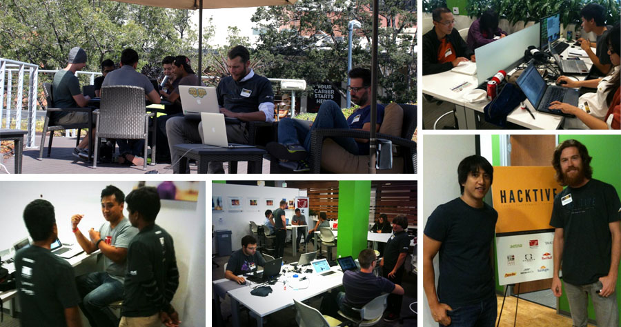
Hackers were doing everything they could to stay awake and comfortable through the 24-hour competition. As the hours passed, snuggies and onesies were used to keep comfy, while others decided to load up on cardiac arrest-enducing amounts of energy drinks. 

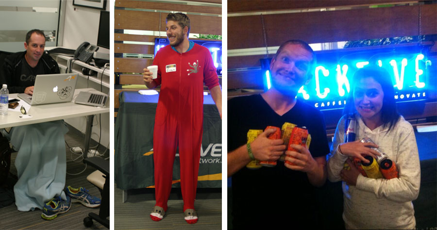
The hackathon proved too much for event emcee, Jon Christopher. He couldnt hack it and fell asleep under the warm glow of the neon HACKTIVE sign. HACKTIVE coach, Cheston Contaoi, and hacker, Eric Johnson, balanced Oreo cookies on thier faces just for fun. Watch the video to find out what really happened - Cheston & Eric. There was even a visit from the ghost of HACKTIVE future. There were a few teams that continued to hack all through the night without any shut-eye. 

On Sunday morning, teams begin to focus on finishing up their apps and preparing their presentations. At noon, the contestants presented their apps to the judges. There was an interesting mix of ideas, from getting gamers more active to using activity data to make romantic connections. Winners included:

ACTIVE Staff:

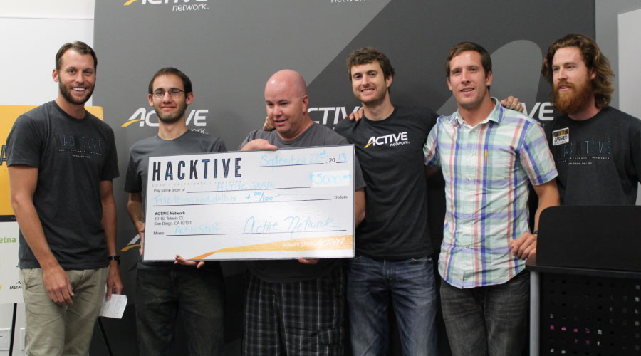
• 1st place: ACTIVE Graph

• Created by Tyler Clemens, Eric Johnson, Trey Gorman & Kevin Brinkley (from left to right in photo below). Social networks like Facebook are mapping the social graph.  ACTIVE Network has the ability to take this a step further and map the activity graph--the relationships between users, their friends, their interests, and the activities in which they participate. Making this graph available across the organization as an enterprise service, using a graph database like Neo4J, opens up a whole new category of connections that can be explored.  Two applications of the graph were demonstrated:  1) recommending networking or meet-up opportunities at an event based on these connections and 2) making targeted event recommendations to users based on friends' interests and activities. Mapping these new connections allows event organizers, media, and ACTIVE Network the ability to leverage this new data to create valuable market opportunities across all of ACTIVE’s platforms. 
• 

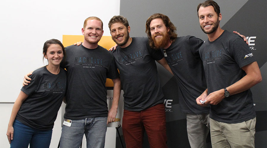
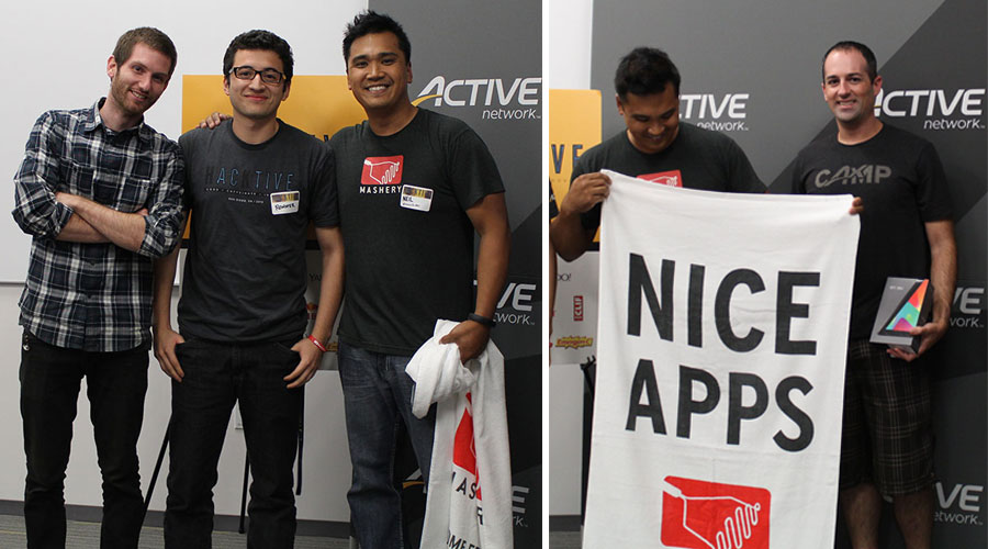
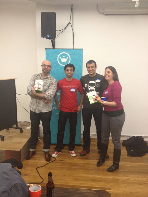
• 2nd place: Spark

• Created by Caitlin Goldman, Jared Planter & Evan Witte (from left to right in photo below). Spark YOUR Training, Spark YOUR Life. This app allows users to create a profile, add interests and event history, and search for events using ACTIVE’s Activity Search API. It gives you the ability to connect with other users that have similar interests and automatically drives romantic connections based on your ‘spark’ potential. Based on the average user spend in the online dating community, this has huge market value if executed correctly.
• 

• 3rd place: ACTIVE Analyze

• Created by Bob Charapata, Daniel Middleton, Jeff Sample & Ryan Sappenfield (no photo, remote team). An Active Network Intranet web application leveraging Microsoft SharePoint self-service business intelligence tools to analyze obesity rates vs. activity participation and other health data. The application queries, in real-time, Active and Mashery API's to return results that are then transformed and loaded into a data model. Users can then create reports and visualizations using a variety of end user BI tools, including; Excel, Power View, Power Pivot and a new Power Map 3D map tool. This data can be used to find new business insights and market opportunities for ACTIVE Network.

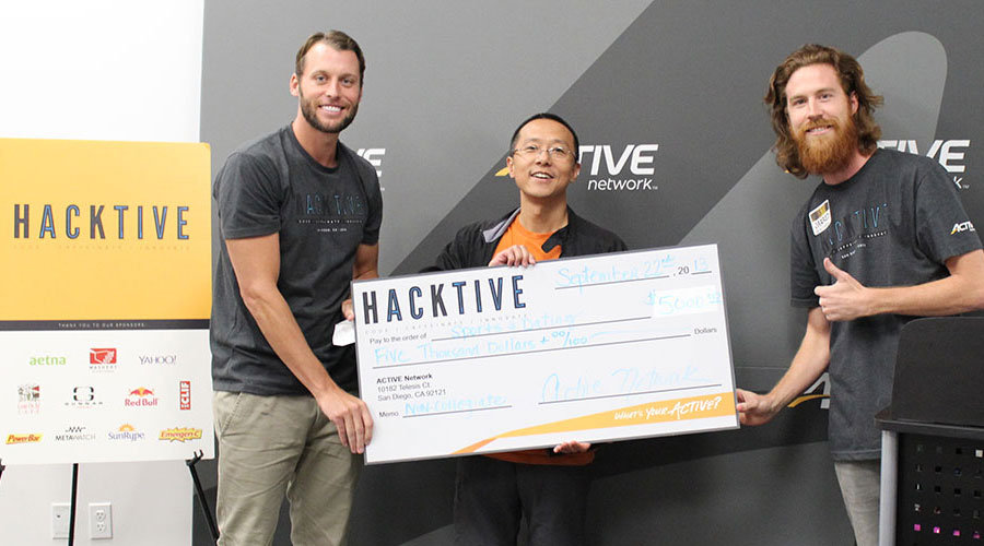
Non-Collegiate:

• 1st place: Sports & Dating

• Created by Bo Li. Sports & Dating is an activity-based dating app, matching singles through sports. Presents your favorite sporting events in the map via the ACTIVE Activity Search API, see how many potential matches have joined the event, then see who is going to the event you are interested in and connecting with others. This app will help to make a dating decision easy and instantly. This will also maximize your chance of meeting someone at an event.
• 

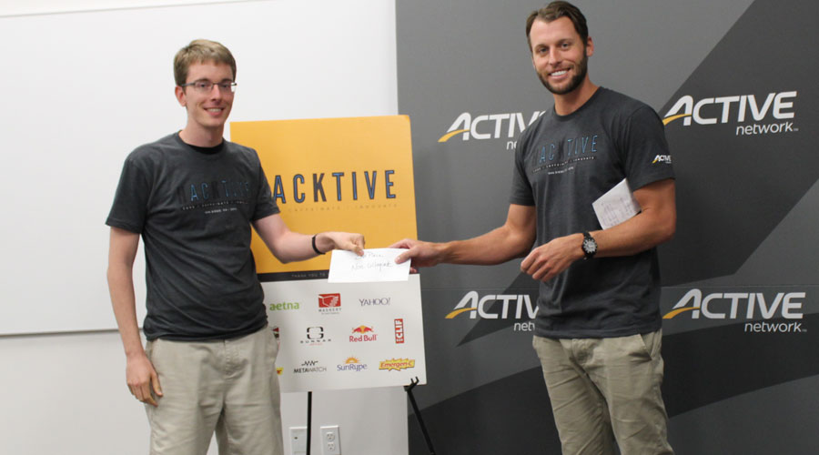
• 2nd place: Get me ACTIVE!

• Created by Joel Drotleff. Fully native iOS 7-optimized app to help people search for activities near them, such as biking, little league, running, and more. Makes it easy to visualize events with topic icons on a map (i.e. runner icon for running type events). Once the user has been to an event, they can reward themselves with a badge and picture to remember their accomplishment. 
• 

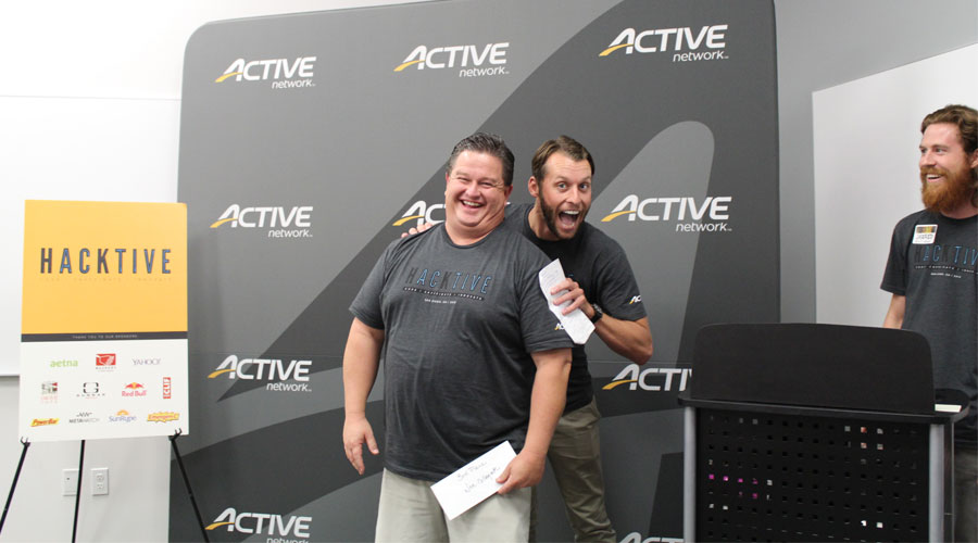
• 3rd place: Phat ACTIVE

• Created by Bret Stateham. Allows users to find events, invite their friends, and then challenge them to a distance run prior to the event. Integrates fitness tracking devices to track challenges prior to the event.
• 

Collegiate:

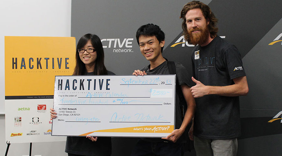
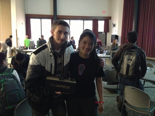
• 1st place: ACTIVE Calendar

• Created by Hoa Mai & Nhu-Quynh Liu. Active Calendar allows the user to search for active events on specific dates by simply clicking a day and entering their search keywords. Future plans to integrate external calendars (iCal, Google Calendar, etc) to allow users to plan their activities around their busy lives.
• 

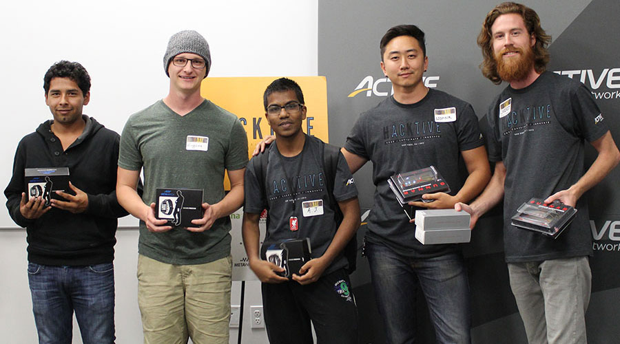
• 2nd place: ActiBar

• Created by Pablo Jacome, Yevgeniy Galipchak, Atyansh Jaiswal, Wonsik Min & Alexander Saavedra (from left to right in photo below - Alexander Saavedra was unable to attend the demo). A simple browser add-on or application that makes it easier for the user to find local physical activities that may range from marathon runs, to simple pickup games in various sports. The user will be able to customize their news feed of activities through a series of personalization questionnaires, in which different activities will be presented depending on the time and location of the user.
• 

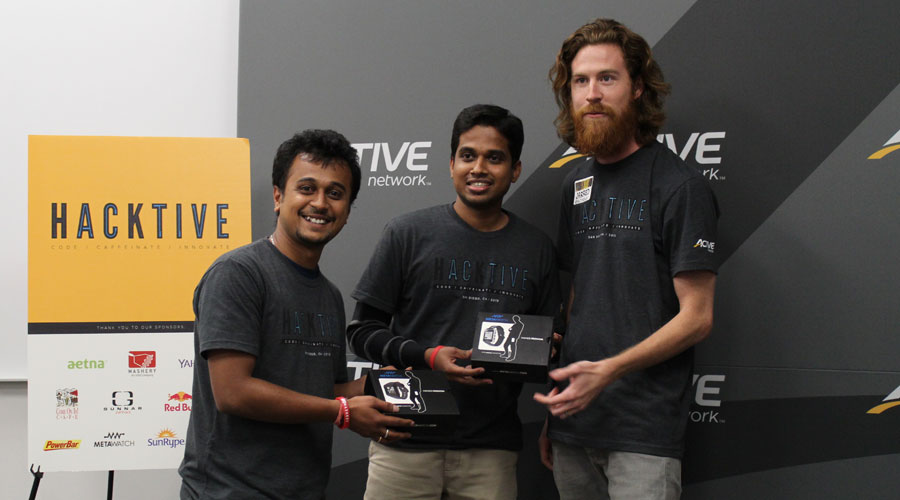
• 3rd place: ACTIVE IT

• Created by Vyshakh Babji & Bharath MylarappaConnect with people around you instantly. Match your interests, contact people in realtime and have fun. Sends an SMS text message when other users signup and select a similar event in your area. Be ACTIVE with others!!!
• 

Mashery Prize:

• The Mashery Prize was won by & Ronad Castillo for effectively using one of the Mashery API Network APIs to build ACTIVEnieghbor - an app that allows users to connect with like-minded individuals within a certain radius that share a similar fitness goal and schedule a time to workout. User-created events are mixed with ACTIVE Network's events and users are gouged into persistent/anonymous chat to discuss goals and schedule a time to train. The app notifies all users and schedules the events on their calendars allowing for organic social growth based on proximity.
• Aaron Waldman also won the Mashery Prize for creating the ACTIVE Leaderboard. His app takes a new look at race results. Now organized into a leaderboard with the users Facebook friends, pulling in their race results for comparison. Now you can compare your fastest 5k against your friends, or at the same event.
• 

You can view all the app submissions online at ChallengePost.

Special thanks the sponsors of the event and the guest judges, Erik Suhonen, Jesse Givens, Neil Mansilla, Tom Clancy, and Mark Roebke for offering your expertise and guidance. Of course, a huge thanks to everyone that participated! We couldn't have made the event a success without the hackers. This beta event gave us a lot of key learnings that will allow us to replicate the model and host a global hackathon in the future.  

You can view all the photos and videos here: http://www.flickr.com/photos/103184269@N08/

HACKTIVE, ACTIVE Network’s first public hackathon, officially opens its doors in less than two weeks. The 24-hour event will take place September 21st, 2013 to September 22nd, 2013 at Co-Merge in San Diego, California. Developers, designers and entrepreneurs will mashup the ACTIVE APIs along with other datasets as they innovate ways of using technology to connect people with activities and ultimately make the world a healthier place.

In addition to being a breeding ground for innovation and inspiration, the hackathon offers attendees the chance to help make a difference, flex their skills, and compete for over $15k in prizes! Here’s just a taste of what participants have in store:

• Two days of intensive collaboration, creativity and caffeination
• An abundance of food, drinks, snacks, and caffeine…thanks to our awesome sponsors
• Feedback from industry experts in both the local and national tech community
• Inspiring keynote along with exciting live demos
• On-site mentoring from passionate hackathon coaches
• HACKTIVE t-shirt to score some street cred
• Opportunity to network with accomplished developers as well as up-and-coming tech talents
• In-person tech support to help troubleshoot
• Fun and energizing interludes plus some sweet swag giveaways

After the submission phase is complete, teams will have three minutes to present their app. Winning hacks will be determined based on four equally-weighted criteria including design, effective use of the ACTIVE Network platform, utility, and originality of concept.  Demos take place in two rounds, where the top teams will advance and battle it out before a panel of industry experts. Here’s a glimpse at the lineup:

	Erik Suhonen - Head of Yahoo! Developer Network, Yahoo!	Erik is responsible for managing a vibrant, global ecosystem of 600,000+ technology companies who engage with Yahoo!'s 30+ platforms.
	Neil Mansilla - Director of Developer Platform & Partnerships, Mashery	Neil is a passionate software engineer and responsible for helping developers discover, learn and utilize the APIs on the Mashery API network.
	Jesse Givens – Head of Product for CarePass, Aetna	With CarePass, Aetna offers all consumers a solution to achieve their unique wellness goals by connecting to top mobile apps.

It’s not too late to sign up, so make arrangements to meet us there!  Register Now: http://developer.active.com/hackathon_2013

Follow us on Twitter @activeapi for the latest event updates!

HACKTIVE is less than a month away, and we couldn’t be more excited for this 24-hour frenzy of coding, collaboration, and caffeine! While this may be ACTIVE Network’s first public hackathon, when it comes to the ACTIVE API, this ain’t its first rodeo. In fact, the Activity Search API has been used to build award-winning apps at numerous hackathons this year alone. Mashery has covered a few of them including last week’s MoDev Hackathon in Seattle, where Bethany Rents (@bethanyrentz) used the Activity API to build her prizewinning app. Built in C# for Windows tablets, To the Finish transforms the experience of training for a marathon or any running event into a social one.

Back in April, two Rutgers students took the title for “Best Use of an API from the Mashery Network,” at the 24-hour student hackathon, HackRU. “Let’s Plan Gen!” built by Joyce Wang and Nikolay Feldman, is an android app that connects users to local happenings, saves ones of interest, and then creates a schedule based on the user's selections. The duo “decided to choose Active because sports activities around the area are not always well-known and publicized enough.” Without any prior experience doing Android programming, both Wang and Feldman found the ease and efficiency of the Activity Search API to be a key component of their success.

And who could forget CouchCachet—the most convenient way of fooling your friends into thinking you’re cooler than you actually are. The mobile app was the Mashery grand prize winner at the foursquare hackathon earlier this year, and created with the help of (wait for it...) the Activity Search API. Harlie, CouchCachet developer explained “CouchCachet allows you to pretend you have a life by checking you in around town while you're still at home.  We then send you a follow up email the next day which contains suggestions for real activities you may want to try doing.  We used your ACTIVE API to populate this email.  It was super easy to use (thanks!) and helped us win the NYC Mashery prize... and were featured in PandoDaily." The team was awarded the opportunity to attend SXSW Interactive and showcase their app in the center ring at Circus Mashimus.

If you haven’t done so already, you should make plans to join us next month at HACKTIVE. Not only will you be competing for a worthy cause, but you’ll also get to hack against the new Activity Search API v2! Now, developers have access to even more events as well as additional flexibility in how they retrieve the data. No matter your skill level, sign up and take part in the awesome innovation happening over the weekend of September 21st-22nd.

We’ll see you in San Diego!

For more information on HACKTIVE or to register, visit http://developer.active.com/hackathon_2013.

Now that registration is officially open for HACKTIVE, our upcoming hackathon event, time is of the essence. With only 24 hours to build your app, how you prepare can make or break your chance at the podium. If you plan to join us this September or are gearing up for another event, there are several measures you can take to maximize your chance at success once the clock starts ticking. Past hackathon champs offer up some of their winning tips:

• Book early. Have you already registered for HACKTIVE? If so, you’re off to a good start. Despite the upsurge in hackathons happening around the globe, it’s not unusual for events to fill up soon after they are announced.

• Find libraries in a language you’re comfortable with. “Sometimes API providers aggregate these on their developer site, but searching github usually does the trick too,” explains Microsoft technical evangelist, Stacey Mulcahy.

• Carefully review the available data sets. Mulcahy also advises developers to “find obscure or interesting API that has lots of data – it will give you more options than an API that has limited endpoints and data.”

• Make lists. “Have a list of interesting data sources, tools, and ideas before going into a hackathon,” suggests Dan Schultz, creator of the winning hack at the recent Knight-Mozilla Open News Hack Day event. “You can use these to brainstorm new ideas with a team, or just pick a single mission and run with it."

• Mitigate against an unstable API that could possibly jeopardize your presentation. Winner of two hackathons, James Rutherford, uses his past failure as an example for why it’s important to plan for the worst. “If you see this is a risk, you have the time, and it suits the scope, then you could mock up some quick and dirty fake local stubs to mimic the API. It’s worth your while capturing some API responses during the event for appropriate endpoints so you can swiftly cludge this if pushed.”

• Take into account how interoperable the API is. Rutherford also recommends to “take time out early on to take a close look at the responses from the APIs, to ensure they’re all usable. For example, there are a raft of ways to specify geolocations – you should ensure that the data formats match the other intended APIs and presentation layers (e.g. map visualisations), or at the least- that you can afford the time to convert between them.”

• Know the access limitations. A final piece of advice from Rutherford cautions developers to be cognizant of the API request rates and any other types of restrictions they may have. “Some have daily limitations, which could hamper the completion of your project at a late stage- local mockups would be useful here too.”

Check out the full article on Programmable Web: Advice from Hackathon Winners: How to Plan Your Time and Choose the Right APIs

Have you participated in a hackathon before? If so, share some of your tips in a comment below!